Obtaining T cells instance labels

from tifffile import imread, imwrite
from pathlib import Path
import napari
import numpy as np
from skimage.io import imread
import napari
import matplotlib.pyplot as plt
# Load image and mask
image_path = "Series003_cCAR_tumor.tif"
mask_path = "masked_predictions.tiff"
image = imread(image_path)  # Expecting shape: (H, W, C)
mask = imread(mask_path)    # Expecting shape: (H, W)
print(f"Image shape: {image.shape}")
print(f"Mask shape: {mask.shape}")

# Create Napari viewer
viewer = napari.Viewer()

# Add the binary mask
viewer.add_image(mask, name='Mask', colormap='grey', blending='additive', opacity=0.5)

# Apply mask to each channel
masked_image = image * mask[..., np.newaxis]  # shape: (H, W, C)

# Split and add each channel separately
colormaps = ['gray', 'green', 'blue', 'magenta']
channel_names = ['Channel 1', 'Channel 2', 'Channel 3', 'Channel 4']
for i in range(masked_image.shape[-1]):
    viewer.add_image(
        masked_image[..., i],
        name=channel_names[i],
        colormap=colormaps[i],
        blending='additive',
        opacity=0.75
    )

napari.run()
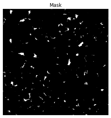
# Normalize mask to be between 0 and 255

plt.imshow((mask * 255).astype(np.uint8)[55], cmap='gray')
plt.title('Mask')
plt.axis('off')
plt.show()

Image shape: (162, 1412, 1412, 4)
Mask shape: (162, 1412, 1412)

Smoothing and spliting of cells

We obtain a mask that doesn’t necessarly posses a cell shape. And we potentially need to split those connected pixels between multiple cells. For that we want to use voronoi_otsu_labeling in order to smooth the mask which will generate elipse (cell shape) and split the connected pixels of the mask between diffrent cells.

# Add new cell with imports
import pyclesperanto_prototype as cle
from skimage.transform import resize
import matplotlib.pyplot as plt

# Initialize GPU (add this in a new cell)

# Add processing cell
def process_tcell_mask(mask_data, spot_sigma=1, outline_sigma=1):
    """Process T-cell mask using Voronoi-Otsu labeling"""
    # Push mask to GPU
    mask_gpu = cle.push(mask_data)
    
    # Apply Voronoi-Otsu labeling
    segmented = cle.voronoi_otsu_labeling(mask_gpu, 
                                         spot_sigma=spot_sigma, 
                                         outline_sigma=outline_sigma)
    
    return segmented

# Add visualization cell
def visualize_segmentation(original_mask, segmented_mask):
    """Visualize original and segmented masks"""
    fig, axs = plt.subplots(1, 2, figsize=(15, 15))
    
    # Original mask
    axs[0].imshow(original_mask, cmap='gray')
    axs[0].set_title('Original Mask')
    axs[0].axis('off')
    
    # Segmented result
    cle.imshow(segmented_mask, labels=True, plot=axs[1])

    axs[1].set_title('Voronoi-Otsu Segmentation')
    axs[1].axis('off')
    
    plt.tight_layout()
    plt.show()

# Add processing execution cell
# Use your existing mask data

# Process each frame if it's a time series
masked_image_one_chanel = masked_image[..., 0]
if len(masked_image_one_chanel.shape) > 2:
    # Process first frame as example
    segmented = process_tcell_mask(masked_image_one_chanel[42])
    visualize_segmentation(masked_image_one_chanel[42], segmented)
else:
    # Process single frame
    segmented = process_tcell_mask(masked_image_one_chanel)
    visualize_segmentation(masked_image_one_chanel, segmented)

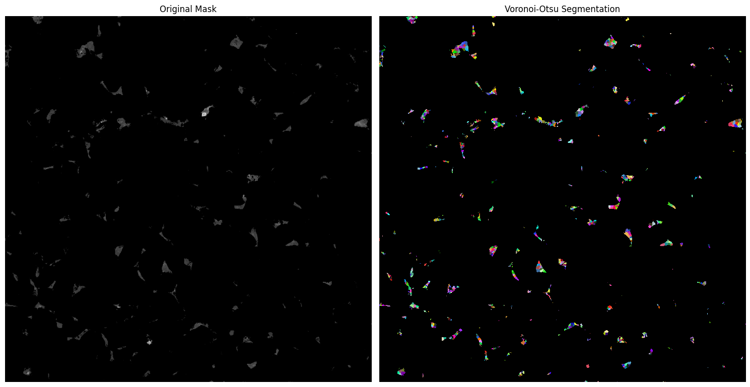
That’s better. However, we need to adjust two parameters correctly: spot_sigma and outline_sigma.

• spot_sigma controls the number of cells detected within a continuous marked pixel zone.
  Increasing spot_sigma results in fewer detected cells, as the algorithm merges more neighboring pixels into a single cell.

• outline_sigma affects the smoothing of the image.
  A higher outline_sigma value produces smoother shapes and outlines by applying more aggressive image smoothing.

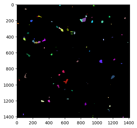
# Test different parameters
spot_sigmas = [6]
outline_sigmas = [4]

for spot_sig in spot_sigmas:
    for outline_sig in outline_sigmas:
        segmented = process_tcell_mask(masked_image_one_chanel[88],
                                     spot_sigma=spot_sig,
                                     outline_sigma=outline_sig)

        # Segmented result
        cle.imshow(segmented, labels=True)
        plt.show()
            

# Test different parameters
spot_sigmas = [6]
outline_sigmas = [2]
for i in range(masked_image_one_chanel.shape[0]):
    for spot_sig in spot_sigmas:
        for outline_sig in outline_sigmas:
            segmented = process_tcell_mask(masked_image_one_chanel[i],
                                         spot_sigma=spot_sig,
                                         outline_sigma=outline_sig)

The post processing is done!!

import matplotlib.colors as mcolors

def generate_unique_colors(segmented_data, background_value=0):
    """Generate unique colors for each unique value in the segmented data."""
    unique_values = np.unique(segmented_data)
    unique_values = unique_values[unique_values != background_value]  # Exclude background value

    color_map = {}
    for value in unique_values:
        # Hash the value to generate a unique color
        np.random.seed(value)  # Use the value as the seed for reproducibility
        color = np.random.rand(3)  # Generate random RGB values
        color_map[value] = mcolors.to_hex(color)  # Convert to hex color

    return color_map

# Generate unique colors for the segmented data
segmented_values = segmented.get()  # Assuming `segmented` is a GPU array, fetch it to CPU
color_map = generate_unique_colors(segmented_values)

# Display the color map
for value, color in color_map.items():
    print(f"Value: {value}, Color: {color}")

Value: 1, Color: #6ab800
Value: 2, Color: #6f078c
Value: 3, Color: #8cb54a
Value: 4, Color: #f78cf8
Value: 5, Color: #39de35
Value: 6, Color: #e455d1
Value: 7, Color: #13c770
Value: 8, Color: #dff7de
Value: 9, Color: #03807e
Value: 10, Color: #c505a2
Value: 11, Color: #2e0576
Value: 12, Color: #27bd43
Value: 13, Color: #c63dd2
Value: 14, Color: #83c5de
Value: 15, Color: #d82e0e
Value: 16, Color: #39858c
Value: 17, Color: #4b8731
Value: 18, Color: #a681e0
Value: 19, Color: #19c23f
Value: 20, Color: #96e5e3
Value: 21, Color: #0c4ab8
Value: 22, Color: #357b6b
Value: 23, Color: #84f1c3
Value: 24, Color: #f5b2ff
Value: 25, Color: #de9447
Value: 26, Color: #4f84c4
Value: 27, Color: #6dd0bc
Value: 28, Color: #ba8f20
Value: 29, Color: #dc4913
Value: 30, Color: #a461a9
Value: 31, Color: #49f4c4
Value: 32, Color: #db5f8e
Value: 33, Color: #3f7369
Value: 34, Color: #0ac718
Value: 35, Color: #754f3b
Value: 36, Color: #ba99f3
Value: 37, Color: #f17631
Value: 38, Color: #62dbf1
Value: 39, Color: #8bcbd1
Value: 40, Color: #680ec9
Value: 41, Color: #400cad
Value: 42, Color: #60f2bb
Value: 43, Color: #1d9b22
Value: 44, Color: #d51bbe
Value: 45, Color: #fc8c48
Value: 46, Color: #c8a240
Value: 47, Color: #1df8ba
Value: 48, Color: #04e349
Value: 49, Color: #4d3fec
Value: 50, Color: #7e3a41
Value: 51, Color: #ac0b58
Value: 52, Color: #d20736
Value: 53, Color: #d88f74
Value: 54, Color: #6b5d2f
Value: 55, Color: #18f87b
Value: 56, Color: #fb55ac
Value: 57, Color: #163b69
Value: 58, Color: #5d737e
Value: 59, Color: #ec28dd
Value: 60, Color: #4d3052
Value: 61, Color: #d22ee0
Value: 62, Color: #097dd8
Value: 63, Color: #8d650c
Value: 64, Color: #619198
Value: 65, Color: #380849
Value: 66, Color: #27225c
Value: 67, Color: #8bdbaf
Value: 68, Color: #420b94
Value: 69, Color: #4cce59
Value: 70, Color: #edde95
Value: 71, Color: #2f63d4
Value: 72, Color: #1baf88
Value: 73, Color: #a48983
Value: 74, Color: #34c8db
Value: 75, Color: #9111e2
Value: 76, Color: #4fd155
Value: 77, Color: #eaa4c0
Value: 78, Color: #0caecc
Value: 79, Color: #807780
Value: 80, Color: #85b245
Value: 81, Color: #5b57ee
Value: 82, Color: #46a39f
Value: 83, Color: #42aea9
Value: 84, Color: #0c5e3e
Value: 85, Color: #9e824c
Value: 86, Color: #343527
Value: 87, Color: #a7f3f8
Value: 88, Color: #a58187
Value: 89, Color: #7f4142
Value: 90, Color: #2728fb
Value: 91, Color: #33544c
Value: 92, Color: #e2c96c
Value: 93, Color: #9ba84e
Value: 94, Color: #b79bb0
Value: 95, Color: #3a31e2
Value: 96, Color: #37e8d0
Value: 97, Color: #d5f772
Value: 98, Color: #bb914d
Value: 99, Color: #ab7cd3
Value: 100, Color: #8b476c
Value: 101, Color: #849207
Value: 102, Color: #98ac4c
Value: 103, Color: #6e2c2c
Value: 104, Color: #263ace
Value: 105, Color: #1555db
Value: 106, Color: #02f373
Value: 107, Color: #29c090
Value: 108, Color: #3c0994
Value: 109, Color: #9c7db2
Value: 110, Color: #1ea860
Value: 111, Color: #9c2b6f
Value: 112, Color: #60a3f2
Value: 113, Color: #d913e4
Value: 114, Color: #27deec
Value: 115, Color: #32b369
Value: 116, Color: #6059ed
Value: 117, Color: #734c3b
Value: 118, Color: #f0940f
Value: 119, Color: #d87f34
Value: 120, Color: #ad839f
Value: 121, Color: #1c363b
Value: 122, Color: #28b343
Value: 123, Color: #b2493a
Value: 124, Color: #1bbe92
Value: 125, Color: #810fa0
Value: 126, Color: #1b2116
Value: 127, Color: #860a2f
Value: 128, Color: #dd4322
Value: 129, Color: #91449a
Value: 130, Color: #244f8d
Value: 131, Color: #a6f263
Value: 132, Color: #c761d3
Value: 133, Color: #6b211c
Value: 134, Color: #cf72a0
Value: 135, Color: #a95432
Value: 136, Color: #272636
Value: 137, Color: #f117b1
Value: 138, Color: #bfb453
Value: 139, Color: #7dc0ee
Value: 140, Color: #bf1c00

from tqdm import tqdm

def apply_color_map_vectorized(segmented_values, color_map):
    """Apply color map in a vectorized way."""
    # Ensure the color map keys are integers
    keys = np.array(list(color_map.keys()), dtype=int)

    # Convert hex to RGB [0, 1]
    colormap_array = np.array([mcolors.to_rgb(color_map[k]) for k in keys], dtype=np.float32)

    # Build a lookup table
    max_label = segmented_values.max()
    lut = np.zeros((max_label + 1, 3), dtype=np.float32)
    lut[keys] = colormap_array

    # Apply the color map using LUT
    rgb_image = lut[segmented_values]

    return rgb_image

# Apply the color map
colored_segmented_image = apply_color_map_vectorized(segmented_values, color_map)

# Test different parameters
from turtle import color

viewer = napari.Viewer()

for spot_sig in spot_sigmas:
    for outline_sig in outline_sigmas:
        # Add original image to Napari
        viewer.add_image(
            masked_image_one_chanel,
            name='Masked Image',
            colormap='gray',
            blending='additive',
            opacity=1
        )

        # Add unmasked image with enhanced contrast to Napari
        colormaps = ['magenta', 'blue', 'green', 'red']  # Diverse colormaps
        for i in range(image.shape[-1]):
            viewer.add_image(
                image[..., i],
                name=f'Channel {i+1}',
                colormap=colormaps[i],
                blending='additive',
                opacity=0.7
            )

        # Add segmented image to Napari with normalized values
        segmented_normalized = (segmented.astype(float) - segmented.min()) / (segmented.max() - segmented.min())
        viewer.add_image(
            colored_segmented_image,
            name='Segmented Image',
            colormap='viridis',  # Using viridis for better distinction
            blending='additive',
            opacity=0.8
        )

napari.run()